Last Change: 2026-01-14 #JT

Quickstart First Time Use

tip

For detailed understanding of how to use spherene, you can download the examples from Resources and find detail descriptions in the tutorial.

In the first time use or in a new PC, the dashboard login page will automatically pop up with the sdk window. Please login your account and activate your license in the current PC.

tip

Once it is done, please restart Rhino/Grasshopper to ensure that all features are correctly loaded based on your license. The license file will be saved locally and be valid for two months. If your license file is out of date, you will receive the following pop-up windows:

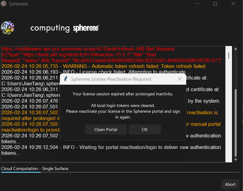
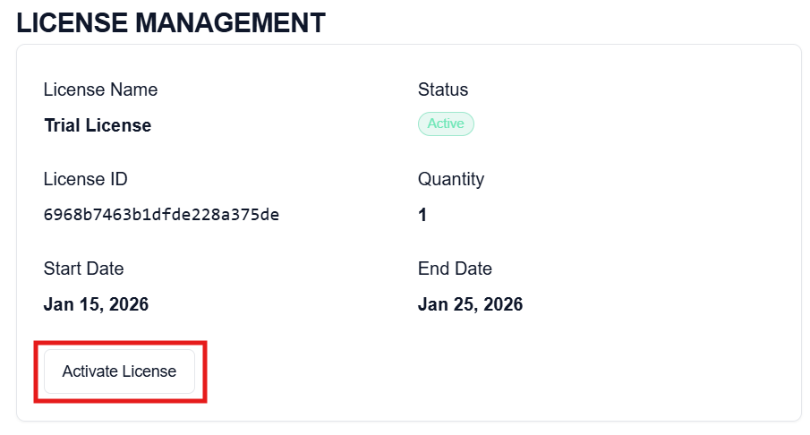
Please then click on "Open portal" and then re-activate your license again in the license management section of your portal dashboard, as shown above.