Last Change: 2026-01-14 #JT
Quickstart First Time Use
This 5-minute video summarizes how to run your first SphereneNTOP computation.
(If you prefer written instructions, please refer to the text-based explanation below.)
UI of Spherene in nTop
In this section, we introduce the user interface of the Spherene connector and explain how to start the Spherene Compute block.
There are two ways to add the Spherene Compute block in nTop:
- Solution 1: Double-click at position 1, type
Create Spherene, and press Enter. - Solution 2: Click the
Create Spherenebutton undernTop > Connectors, as shown in position 2 in the figure below.
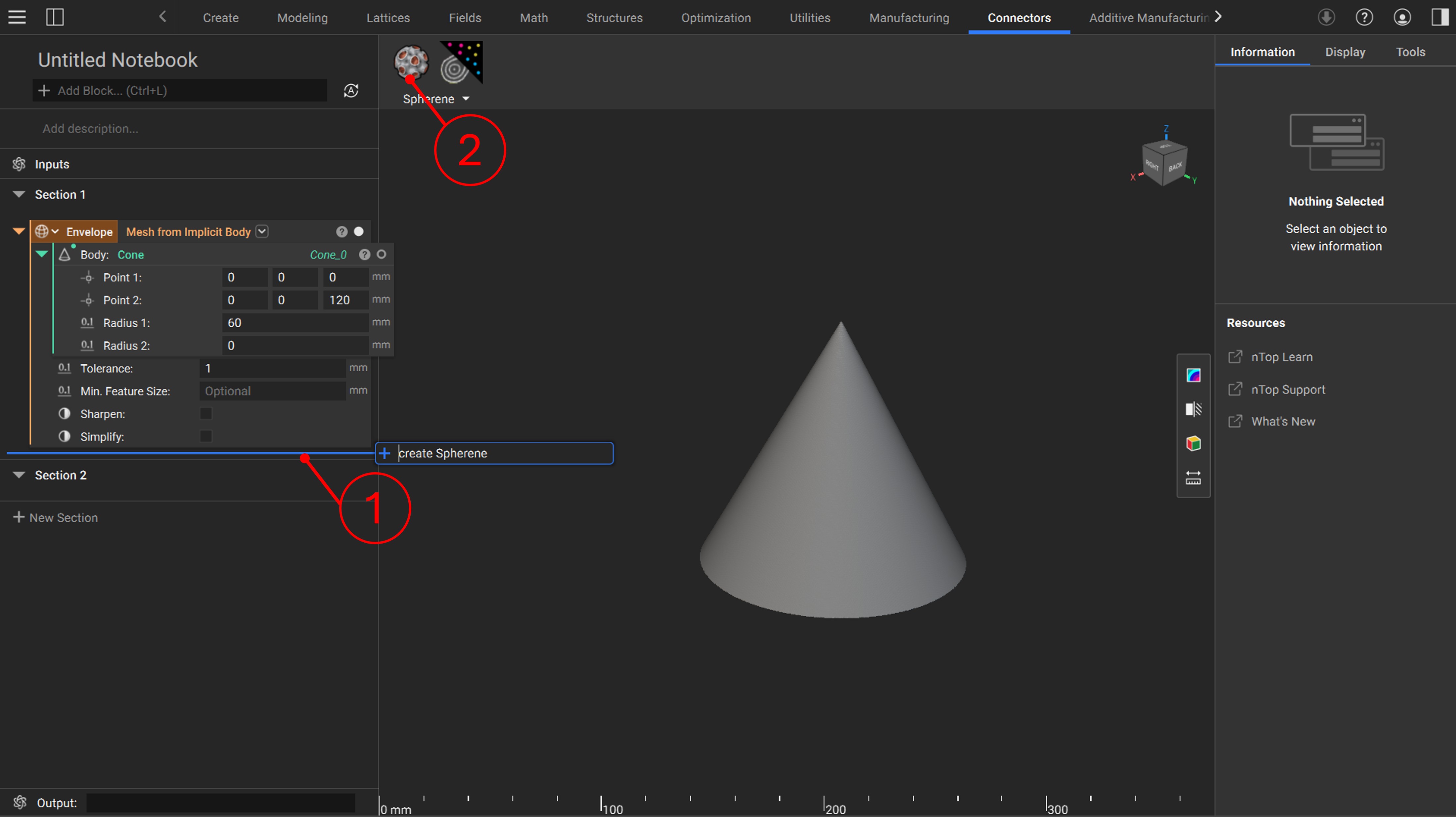
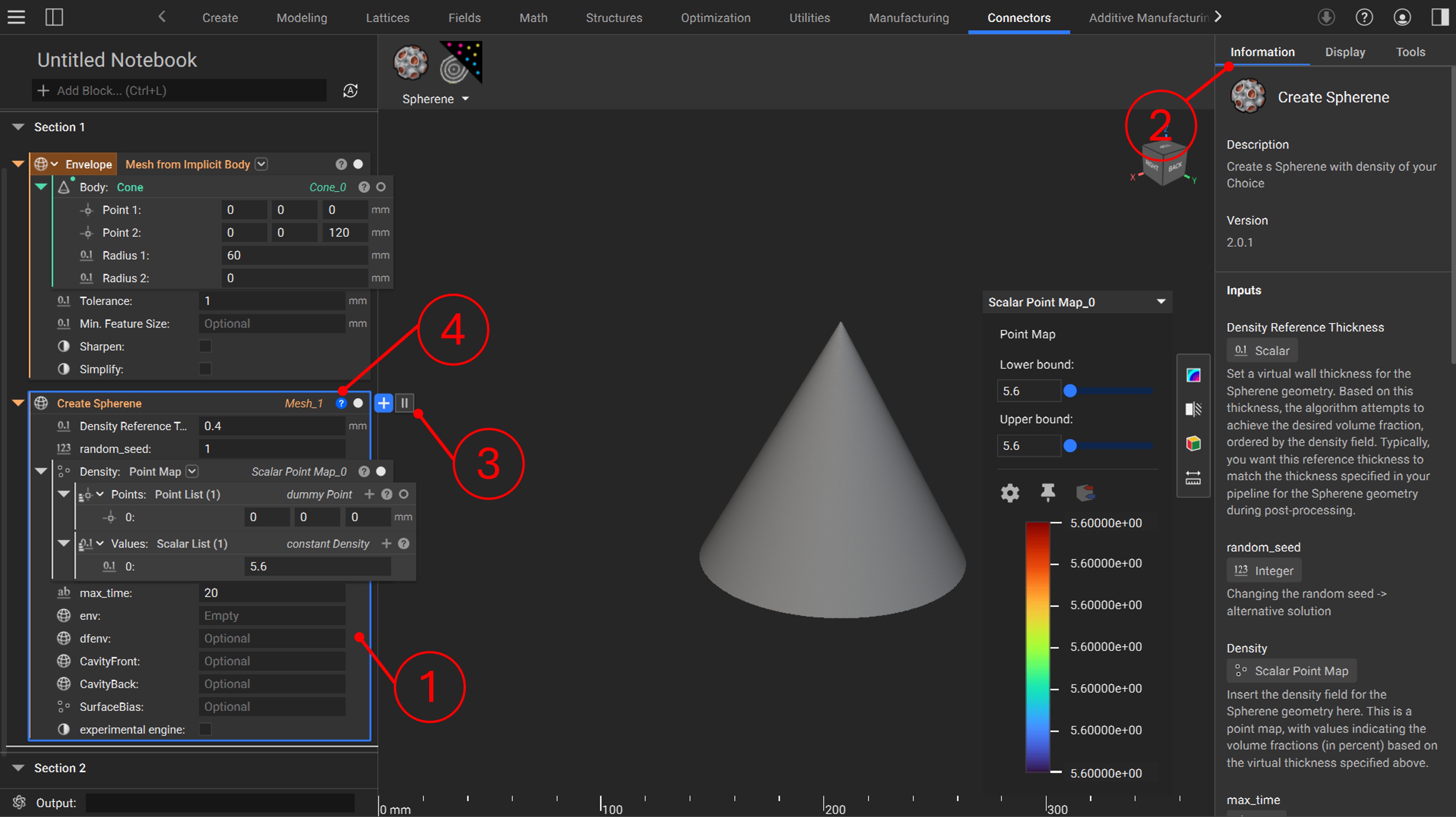
The UI of the Spherene Compute block is shown at position 1 in the figure below. Details for each attribute are displayed in the Information section (position 2).
The first important step after adding the Spherene Compute block is to right-click on the block and set it to Manual Run Mode. This prevents nTop from automatically running the computation every time you change an attribute, saving both computational resources and time. You can find the pause/run button at position 3. To start the computation, please ensure all settings are properly configured. The ? button at position 4 will provide hints if there are any issues with the configuration.
General workflow
The input and output of Spherene compute block are both mesh. To start a spherene computation, you need to first generate a mesh of envelope and feed it into the input Envelope of Create Spherene block. And then you can run the block to start the compute as the simplest setup.
An black sdk window should pop up which tells the computational progression and messages. Each computation consumes a certain number of credits from your account (details see Credit Rules).
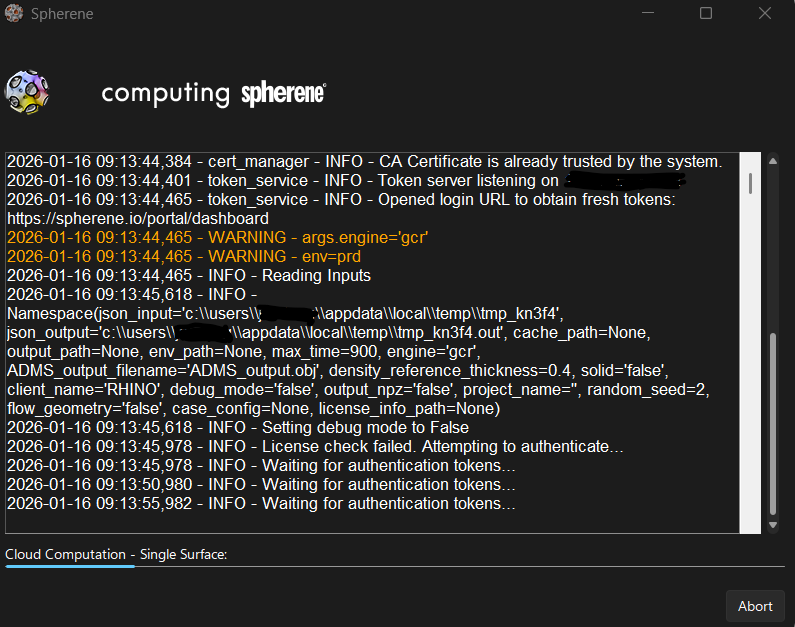
In the first time use or in a new PC, the dashboard login page will automatically pop up with the sdk window. Please login your account and activate your license in the current PC.
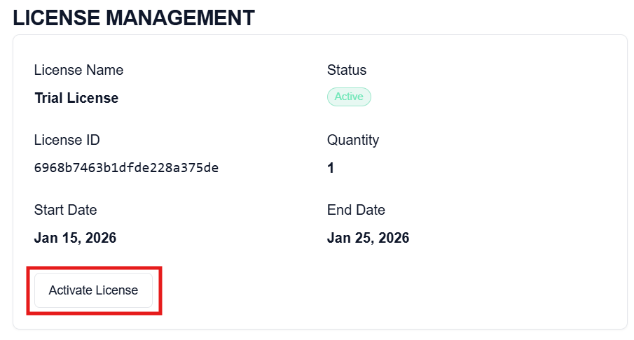
Once it is done, please restart nTop to ensure that all features are correctly loaded based on your license. The license file will be saved locally and be valid for two months. If your license file is out of date, you will receive the following pop-up windows:
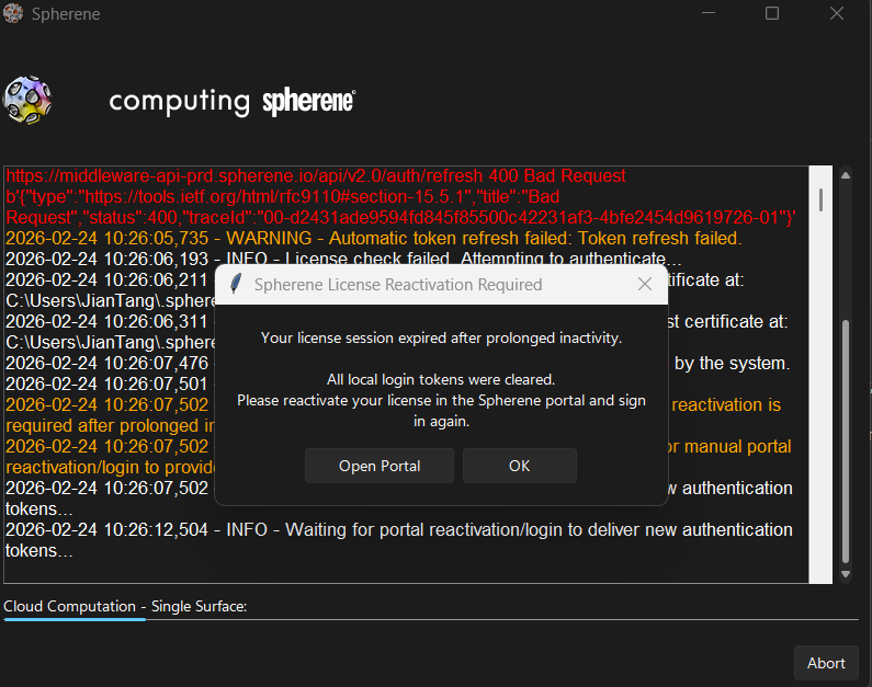
Please then click on "Open portal" and then re-activate your license again in the license management section of your portal dashboard, as shown above.
Save your nTop file before starting a Spherene Computation to avoid "Envelope not Found" warning.
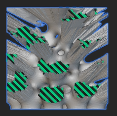
You might get a "open mesh" warning from nTop when the computation finish. Please ignore it. And you will see some nasty artifacts if you create a implicit body from the outputted spherene single-surface mesh. However, these are nTop visualization artifacts. It will go away once you thicken the body.