Last Change: 2026-01-14 #JT
Quickstart First Time Use
This 5-minute video summarizes how to run your first SphereneFusion computation.
(If you prefer written instructions, please refer to the text-based explanation below.)
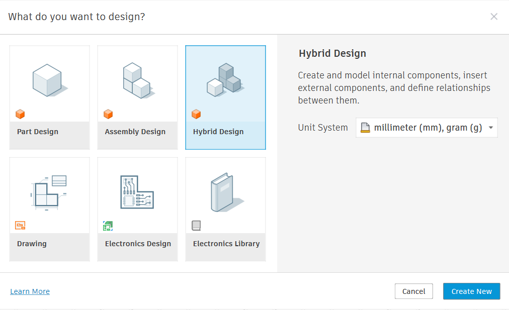
Fusion 360 releases new design templates in January 2026. For Spherene users, we kindly ask you to use the “Hybrid Design” template when creating a new Fusion project.
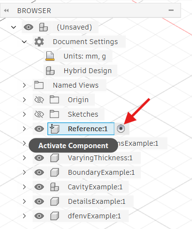
SphereneFUSION treats each component as an individual Spherene project. Therefore, before using Spherene in Fusion, ensure that the envelope geometry of interest is placed inside a component, and activate the corresponding component by clicking the dot next to the component name.
A general workflow of a spherene computation includes three steps:
-
Create a Spherene project and assign an envelope
-
set up spherene related parameters such as thickness and density (details see Tutorial For Basic Features);
-
define output format and computation setting, then start the compute. An black sdk window should pop up which tells the computational progression and messages. Each computation consumes a certain number of credits from your account (details see Credit Rules).
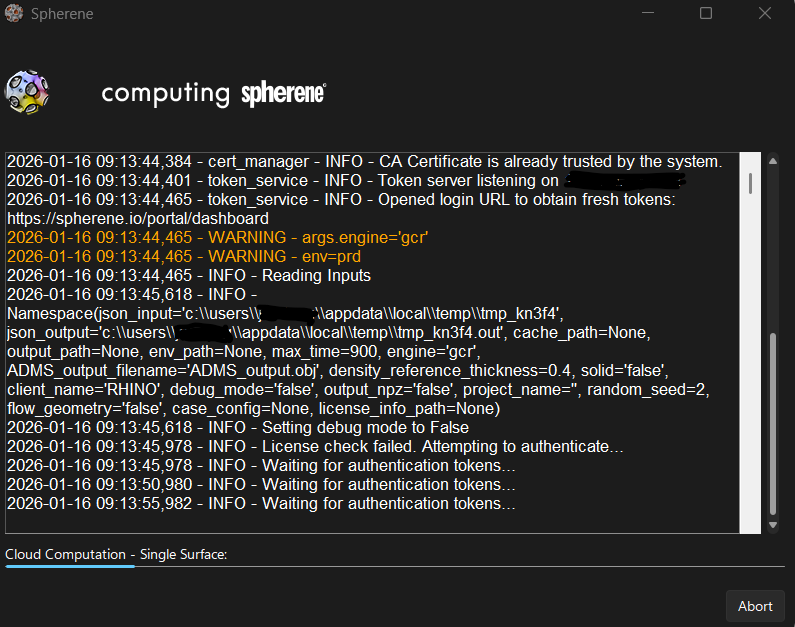
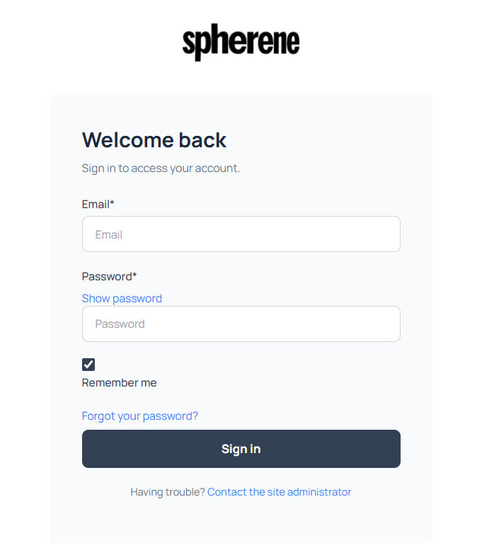
In the first time use or in a new PC, the dashboard login page will automatically pop up with the sdk window. Please login your account and activate your license in the current PC.
 tip
tipOnce it is done, please restart Fusion to ensure that all features are correctly loaded based on your license. The license file will be saved locally and be valid for two months. If your license file is out of date, you will receive the following pop-up windows:
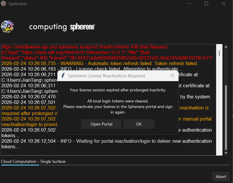
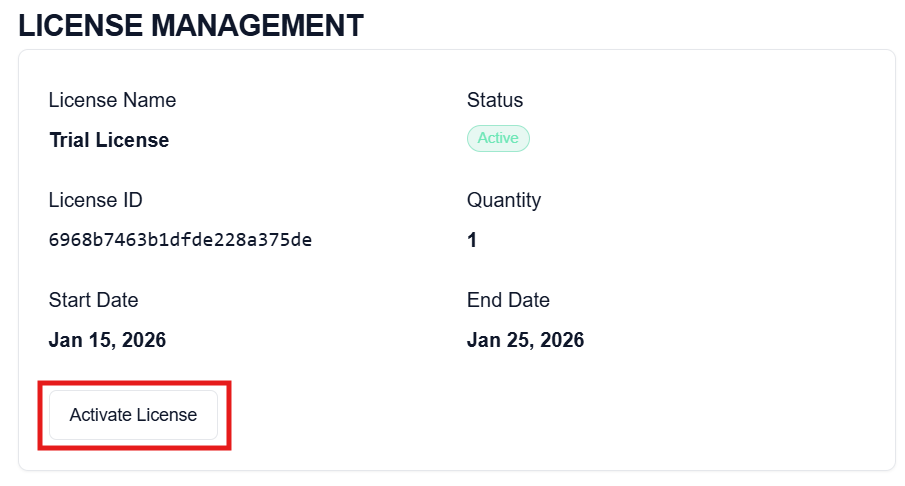
Please then click on "Open portal" and then re-activate your license again in the license management section of your portal dashboard, as shown above.